$\LaTeX{}$之数学公式(四)
本文主体内容来自一份 (不太) 简短的 LATEX2ε 介绍。
本章将见识到 \(\LaTeX{}\) 闻名的强项——排版数学公式。
\(\textrm{AMS}\) 宏集
在介绍数学公式排版之前,简单介绍一下 \(\textrm{AMS}\) 宏集。\(\textrm{AMS}\)
宏集合是美国数学学会(American Mathematical Society)提供的对\(\LaTeX{}\)
原生的数学公式排版的扩展,其核心是 amsmath
宏包,对多行公式的排版提供了有力的支持。此外,amsfonts
宏包以及基于它的 amssymb
宏包提供了丰富的数学符号;amsthm 宏包扩展了 \(\LaTeX{}\) 定理证明格式。
以下示例都假定了导言区中写有 \usepackage{amsmath} 。
公式排版基础
行内和行间公式
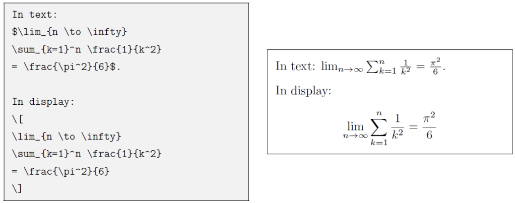
数学公式有两种排版方式:其一是与文字混排,称为行内公式;其二是单独列为一行排版,称为行间公式。
行内公式由一对 \(\texttt\$\)
符号包裹:The Pythagorean theorem is \(a^2 +
b^2 = c^2\) ($a^2 + b^2 = c^2$)。
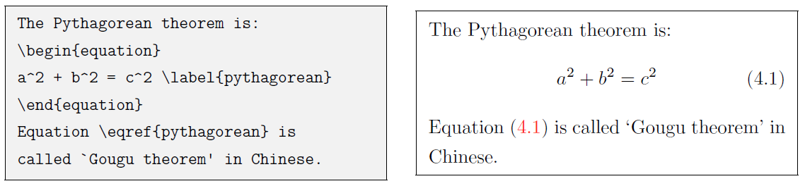
单独成行的行间公式由 \(\texttt{equation}\) 环境包裹。 \(\texttt{equation}\)
环境为公式自动生成一个编号,这个编号可以用\label 和
\ref 生成交叉引用,amsmath 的
\eqref
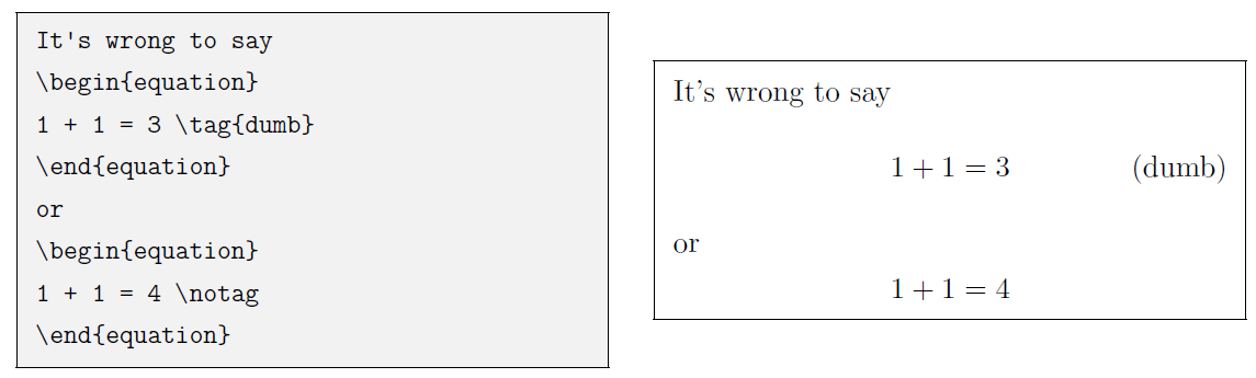
命令甚至为引用自动加上圆括号;还可以用\tag
命令手动修改公式的编号,或者用\notag
命令取消为公式编号(与之基本等效的命令是 \nonumber)。
1 | \begin{equation} |
1 | \begin{equation} |
\[ \begin{equation} 1 + 1 = 3 \tag{dumb} \end{equation} \]
\[ \begin{equation} 1 + 1 = 4 \notag \end{equation} \]
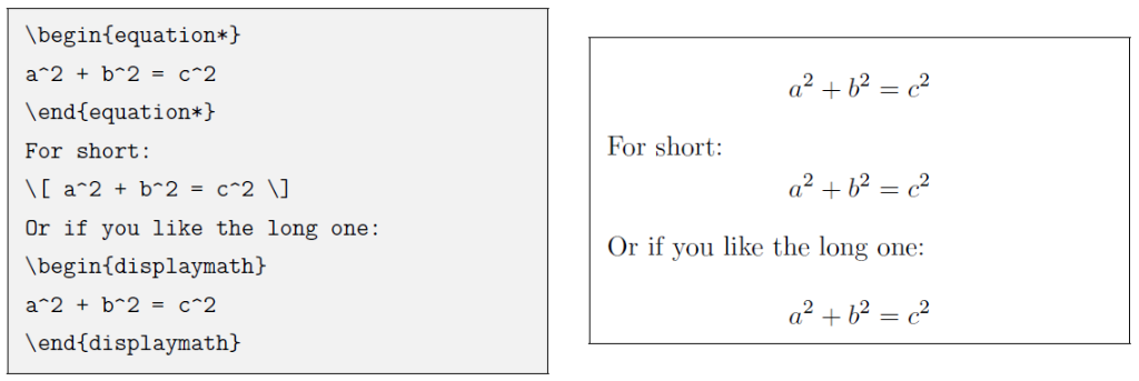
如果需要直接使用不带编号的行间公式,则将公式用命令 \[ 和
\] 包裹,与之等效的是 \(\texttt{displaymath}\) 环境。有的人更喜欢
\(\texttt{equation*}\)
环境,体现了带星号和不带星号的环境之间的区别。
通过一个例子展示行内公式和行间公式的对比。为了与文字相适应,行内公式在排版大的公式元素(分式、巨算符等)时显得很“局促”:
行间公式的对齐、编号位置等性质由文档类选项控制,文档类的 \(\texttt{fleqn}\) 选项令行间公式左对齐;\(\texttt{leqno}\) 选项令编号放在公式左边。
数学模式
当用户使用 \(\texttt\$\)
开启行内公式输入,或是使用 \[ 命令、\(\texttt{equation}\) 环境时,\(\LaTeX{}\)
就进入了数学模式。
数学模式相比于文本模式有以下特点:
- 数学模式中输入的空格被忽略。数学符号的间距默认由符号的性质(关系符号、运算符等)决定。需要人为引入间距时,
\quad和\qquad等命令。- 不允许有空行(分段)。行间公式中也无法用
\\命令手动换行。- 所有的字母被当作数学公式中的变量处理,字母间距与文本模式不一致,也无法生成单词之间的空格。如果想在数学公式中输入正体的文本,简单情况下可用
\mathrm命令。或者用\amsmath提供的\text命令。
1 | $x^{2} \geq 0 \qquad |
\[ \begin{gather*} x^{2} \geq 0 \qquad \text{for \textbf{all} } x\in \mathbb{R} \end{gather*} \]
数学符号
\(\LaTeX{}\)
默认提供了常用的数学符号,amssymb
宏包提供了一些次常用的符号。大多数常用的数学符号都能在 这里
查到。更多符号可在命令行输入texdoc symbols-a4 查阅
。
一般符号
希腊字母符号的名称就是其英文名称,如 \(\alpha\) (\alpha)、\(\beta\)
(\beta)等等。大写的希腊字母为首字母大写的命令 \(\Gamma\) (\Gamma) \(\Delta\)
(\Delta)。无穷大符号为 \(\infty\) (\infty)。
省略号有 \(\dots\)
(\dots) 和 \(\cdots\)
(\cdots) 两种形式。它们有各自合适的用途:
1 | $a_1, a_2, \dots, a_n$ \\ |
\[ \begin{gather*} a_1, a_2, \dots, a_n \\ a_1 + a_2 + \cdots + a_n \end{gather*} \]
\ldots 和 \dots
是完全等效的,它们既能用在公式中,也用来在文本里作为省略号。
除此之外,在矩阵中可能会用到竖排的 \(\vdots\) (\votes)和斜排的
\(\ddots\) (\ddots)。
指数、上下标和导数
用^ 和
_标明上下标。注意上下标的内容(子公式)一般需要用花括号包裹,否则上下标只对后面的一个符号起作用。
1 | $p^3_{ij} \qquad |
\[ \begin{gather*} p^3_{ij} \qquad m_\mathrm{Knuth}\qquad \sum_{k=1}^3 k \\[5pt] a^x+y \neq a^{x+y}\qquad e^{x^2} \neq {e^x}^2 \end{gather*} \]
导数符号'(\({}'\))是一类特殊的上标,可连续使用,但只能在其后添加其他上标:
1 | $f(x) = x^2 \quad f'(x) = 2x \quad f''^{2}(x) = 4$ |
\[ f(x) = x^2 \quad f'(x) = 2x \quad f''^{2}(x) = 4 \]
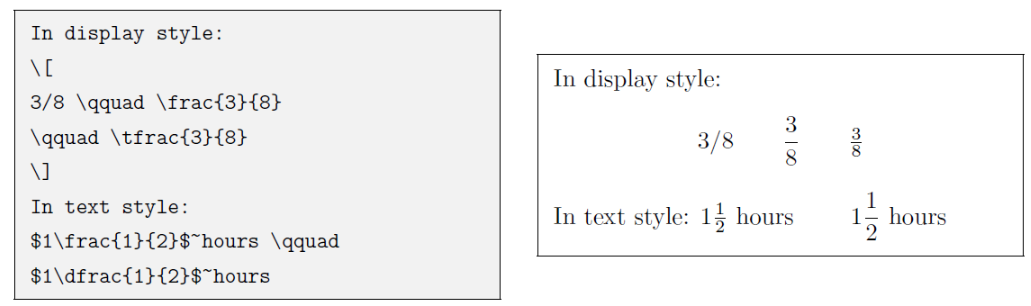
分式和根式
分式使用 \frac{分子}{分母}
来书写。分式的大小在行间公式中是正常大小,而在行内被极度压缩。
amsmath 提供了方便的命令 \dfrac 和
\tfrac,令用户能够在行内使用正常大小的分式,或是反过来。
1 | In display style: |
一般的根式使用 \sqrt{...};表示 \(n\) 次方根时写成
\sqrt[n]{...}。
1 | $\sqrt{x} \Leftrightarrow x^{1/2} |
\[ \sqrt{x} \Leftrightarrow x^{1/2} \quad \sqrt[3]{2} \quad \sqrt{x^{2} + \sqrt{y}} \]
特殊的分式形式,如二项式结构,由 amsmath 宏包的
\binom 命令生成:
1 | \[ |
\[
\binom{n}{k} =\binom{n-1}{k}
+ \binom{n-1}{k-1}
\]
关系符
常见的关系符号除了可以直接输入的 \(=\),\(>\),\(<\),其它符号用命令输入,常用的有 \(\ne\) (\ne)、\(\ge\) (\ge)、\(\le\) (\le)、\(\approx\) (\approx)、 等价
\(\equiv\) (\equiv)、正比
\(\propto\)
(\propto)、相似 \(\sim\)\sim 等等。
\(\LaTeX{}\)
还提供了自定义二元关系符的命令
\stackrel,用于将一个符号叠加在原有的二元关系符之上:
1 | $f_n(x) \stackrel{*}{\approx} 1$ |
\[ f_n(x) \stackrel{*}{\approx} 1 \]
运算符
\(\LaTeX{}\)
中的算符大多数是二元算符,除了直接用键盘可以输入的 \(+\)、\(-\)、\(*\)、\(/\),其它符号用命令输入,常用的有乘号 \(\times\) (\times)、 除号 \(÷\)(\div)、点乘 \(\cdot\) (\cdot)、加减号\(\pm\) (\pm) / \(\mp\) (\mp)等等。
\(\nabla\) (\nabla) 和
\(\partial\) (\partial)
也是常用的算符,虽然它们不属于二元算符。
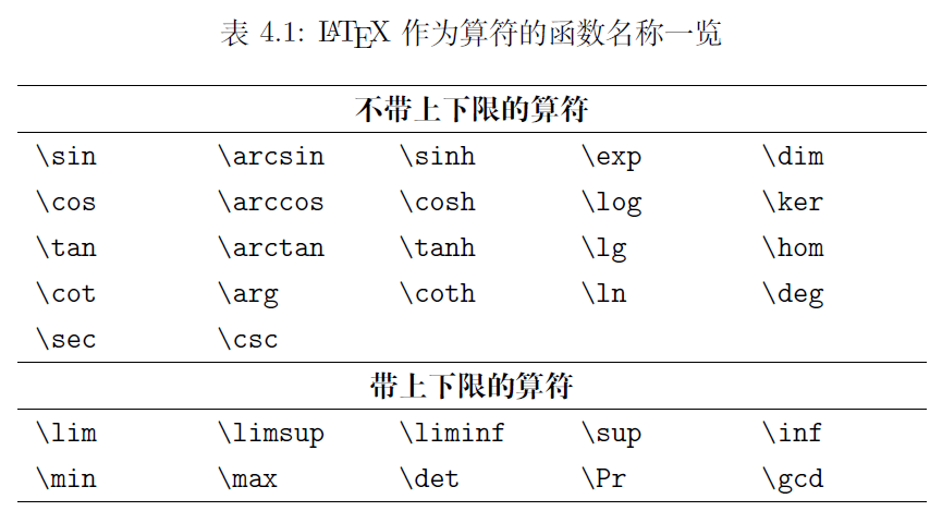
\(\LaTeX{}\) 将数学函数的名称作为一个算符排版,字体为直立字体。其中有一部分符号在上下位置可以书写一些内容作为条件, 类似于后文所叙述的巨算符。
1 | $\lim_{x \rightarrow 0} \frac{\sin x}{x} = 1$ |
\[ \lim_{x \rightarrow 0} \frac{\sin x}{x} = 1 \]
对于求模表达式,\(\LaTeX{}\) 提供了
\bmod和 \pmod
命令,前者相当于一个二元运算符,后者作为同余表达式的后缀:
1 | $a\bmod b \\ |
\[ \begin{gather*} a\bmod b \\ x\equiv a \pmod{b} \end{gather*} \]
如果上表中的算符不够用的话,amsmath 允许用户在导言区用
\DeclareMathOperator定义自己的算符,其中带星号的命令定义带上下限的算符:
1 | \DeclareMathOperator{\argh}{argh} |
\[ \DeclareMathOperator{\argh}{argh} \DeclareMathOperator*{\nut}{Nut} \argh 3 = \nut_{x=1} 4x \]
巨算符
积分号 \(\int\)
(\int)、求和号 \(\sum\)
(\sum)
等符号称为巨算符。巨算符在行内公式和行间公式的大小和形状有区别。行内:\(\sum_{i=1}^n \quad
\int_0^{\frac{\pi}{2}} \quad
\oint_0^{\frac{\pi}{2}} \quad
\prod_\epsilon\) ,行间:
1 | \[\sum_{i=1}^n \quad |
\[ \sum_{i=1}^n \quad \int_0^{\frac{\pi}{2}} \quad \oint_0^{\frac{\pi}{2}} \quad \prod_\epsilon \]
巨算符的上下标位置可由 \limits 和
\nolimits调整,前者令巨算符类似 \(\lim\) 或求和算符 \(\sum\),上下标位于上下方;后者令巨算符类似积分号,上下标位于右上方和右下方。行内:\(\sum\limits_{i=1}^n \quad
\int\limits_0^{\frac{\pi}{2}} \quad
\prod\limits_\epsilon\) ; 行间:
1 | \[\sum\nolimits_{i=1}^n \quad |
\[ \sum\nolimits_{i=1}^n \quad \int\limits_0^{\frac{\pi}{2}} \quad \prod\nolimits_\epsilon \]
amsmath 宏包还提供了
\substack,能够在下限位置书写多行表达式;\(\texttt{subarray}\)
环境更进一步,令多行表达式可选择居中 (c) 或左对齐 (l):
1 | % \usepackage{amssymb} |
\[ \begin{gather*} \sum_{\substack{0\le i\le n \\ j\in \mathbb{R}}} P(i,j) = Q(n) \\ \sum_{\begin{subarray}{l} 0\le i\le n \\ j\in \mathbb{R} \end{subarray}} P(i,j) = Q(n) \end{gather*} \]
数学重音和上下括号
数学符号可以像文字一样加重音,比如求导符号 \(\dot{r}\) (\dot{r})、 \(\ddot{r}\)
(\ddot{r})、表示向量的箭头 \(\vec{r}\) (\vec{r})
、表示单位向量的符号 \(\hat{\mathbf{e}}\)
(\hat{mathbf{e}})等。使用时要注意重音符号的作用区域,一般应当对某个符号而不是“符号加下标”使用重音:
1 | $\bar{x_0} \quad \bar{x}_0$\\[5pt] |
\[ \begin{gather*} \bar{x_0} \quad \bar{x}_0\\[5pt] \vec{x_0} \quad \vec{x}_0\\[5pt] \hat{\mathbf{e}_x} \quad \hat{\mathbf{e}}_x \end{gather*} \]
也能为多个字符加重音,包括直接画线的 \overline 和
\underline 命令(可叠加使用)、宽重音符号
\widehat、表示向量的箭头 \overrightarrow
等。
1 | $0.\overline{3} = \underline{\underline{1/3}}$ \\[5pt] |
\[ \begin{gather*} 0.\overline{3} = \underline{\underline{1/3}} \\[5pt] \hat{XY} \qquad \widehat{XY}\\[5pt] \vec{AB} \qquad \overrightarrow{AB} \end{gather*} \]
\overbrace 和 \underbrace
命令用来生成上/下括号,各自可带一个上/下标公式。
1 | $\underbrace{\overbrace{(a+b+c)}^6 |
\[ \underbrace{\overbrace{(a+b+c)}^6 \cdot \overbrace{(d+e+f)}^7} _\text{meaning of life} = 42 \]
箭头
常用的箭头包括 \rightarrow(\(\rightarrow\),或
\to)、\leftarrow(\(\leftarrow\),或\gets)等。
amsmath 的 xleftarrow 和
xrightarrow
命令提供了长度可以伸展的箭头,并且可以为箭头增加上下标:
1 | \[ a\xleftarrow{x+y+z} b \] \\ |
\[ \begin{gather*} a\xleftarrow{x+y+z} b \\ c\xrightarrow[x<y]{a*b*c}d \end{gather*} \]
括号和定界符
\(\LaTeX{}\)
提供了多种括号和定界符表示公式块的边界,如小括号 \(()\)、中括号 \([]\)、大括号 \(\{\}\) (\{ \})、尖括号 \(\langle \rangle\)(\langle
\rangle)等。
1 | ${a,b,c} \neq \{a,b,c\}$ |
\[ {a,b,c} \neq \{a,b,c\} \]
使用 \left 和 \right
命令可令括号(定界符)的大小可变,在行间公式中常用。会自动根据括号内的公式大小决定定界符大小。
\left 和 \right
必须成对使用。需要使用单个定界符时,另一个定界符写成 \left.
或\right.。
1 | \[1 + \left(\frac{1}{1-x^{2}} |
\[ 1 + \left(\frac{1}{1-x^{2}} \right)^3 \qquad \left.\frac{\partial f}{\partial t} \right|_{t=0} \]
有时我们不满意于 \(\LaTeX{}\)
自动调节的定界符大小。这时还可以用 \big、bigg
等命令生成固定大小的定界符。 更常用的形式是类似 \left 的
\bigl、\biggl 等,以及类似 \right
的 \bigr、\biggr 等(\bigl 和
\bigr 不必成对出现)。
1 | $\Bigl((x+1)(x-1)\Bigr)^{2}$\\ |
\[ \begin{gather*} \Bigl((x+1)(x-1)\Bigr)^{2}\\ \bigl( \Bigl( \biggl( \Biggl( \quad \bigr\} \Bigr\} \biggr\} \Biggr\} \quad \big\| \Big\| \bigg\| \Bigg\| \quad \big\Downarrow \Big\Downarrow \bigg\Downarrow \Bigg\Downarrow \end{gather*} \]
使用 \big 和 \bigg
等命令的另外一个好处是:用\left 和 \right
分界符包裹的公式块是不允许断行的(下文提到的 \(\texttt{array}\) 或者 \(\texttt{aligned}\)
等环境视为一个公式块),所以也不允许在多行公式里跨行使用,而
\big 和 \bigg 等命令不受限制。
多行公式
长公式折行
通常来讲应当避免写出超过一行而需要折行的长公式。如果一定要折行的话,习惯上优先在等号之前折行,其次在加号、减号之前,再次在乘号、除号之前。 其它位置应当避免折行。
amsmath 宏包的 \(\texttt{multline}\)
环境提供了书写折行长公式的方便环境。它允许用 \\
折行,将公式编号放在最后一行。多行公式的首行左对齐,末行右对齐,其余行居中。
1 | \begin{multline} |
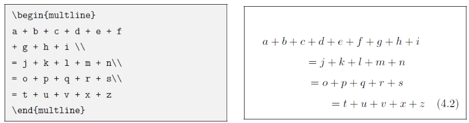
与表格不同的是,公式的最后一行不写
\\,如果写了,反倒会产生一个多余的空行。
类似 \(\texttt{equation*}\),\(\texttt{multline*}\) 环境排版不带编号的折行长公式。
多行公式
更多的情况是,需要罗列一系列公式,并令其按照等号对齐。 目前最常用的是 \(\texttt{align}\) 环境,它将公式用 \(\texttt\&\) 隔为两部分并对齐。分隔符通常放在等号左边:
1 | \begin{align} |
\[ \begin{align} a & = b + c \\ & = d + e \end{align} \]
\(\texttt{align}\)
环境会给每行公式都编号。仍然可以用 \notag 去掉某行的编号。
在以下的例子,为了对齐等号,将分隔符放在右侧,并且此时需要在等号后添加一对括号
\(\texttt\{\texttt\}\)
以产生正常的间距:
1 | \begin{align} |
\[ \begin{align} a ={} & b + c \\ ={} & d + e + f + g + h + i + j + k + l \notag \\ & + m + n + o \\ ={} & p + q + r + s \end{align} \]
\(\texttt{align}\)
还能够对齐多组公式,除等号前的 & 之外, 公式之间也用
& 分隔:
1 | \begin{align} |
\[ \begin{align} a &=1 & b &=2 & c &=3 \\ d &=-1 & e &=-2 & f &=-5 \end{align} \]
如果不需要按等号对齐,只需罗列数个公式,\(\texttt{gather}\) 将是一个很好用的环境:
1 | \begin{gather} |
\[ \begin{gather} a = b + c \\ d = e + f + g \\ h + i = j + k \notag \\ l + m = n \end{gather} \]
有对应的不带编号的版本 \(\texttt{align*}\)和 \(\texttt{gather*}\)。
公用编号的多行公式
另一个常见的需求是将多个公式组在一起公用一个编号,编号位于公式的居中位置。为此,amsmath
宏包提供了诸如 \(\texttt{aligned}\)、\(\texttt{gathered}\) 等环境,与 \(\texttt{equation}\) 环境套用。以 \(\texttt{-ed}\) 结尾的环境用法与前一节不以
\(\texttt{-ed}\)
结尾的环境用法一一对应。仅以 \(\texttt{aligned}\) 举例:
1 | \begin{equation} |
\[ \begin{equation} \begin{aligned} a &= b + c \\ d &= e + f + g \\ h + i &= j + k \\ l + m &= n \end{aligned} \end{equation} \]
\(\texttt{split}\) 环境和 \(\texttt{aligned}\) 环境用法类似,也用于和 \(\texttt{equation}\) 环境套用,区别是 \(\texttt{split}\) 只能将每行的一个公式分两栏,\(\texttt{aligned}\) 允许每行多个公式多栏。
数组和矩阵
为了排版二维数组,\(\LaTeX{}\)
提供了 \(\texttt{array}\) 环境,用法与
\(\texttt{tabular}\)
环境极为类似,也需要定义列格式,并用 \\
换行。数组可作为一个公式块,在外套用
\left、\right 等定界符:
1 | \[ \mathbf{X} = \left( |
\[ \mathbf{X} = \left(
\begin{array}{cccc}
x_{11} & x_{12} & \ldots & x_{1n}\\
x_{21} & x_{22} & \ldots & x_{2n}\\
\vdots & \vdots & \ddots & \vdots\\
x_{n1} & x_{n2} & \ldots & x_{nn}\\
\end{array} \right) \]
值得注意的是,上一节末尾介绍的 \(\texttt{aligned}\) 等环境也可以用定界符包裹。
还可以利用空的定界符排版出这样的效果:
1 | \[ |x| = \left\{ |
\[ |x| = \left\{
\begin{array}{rl}
-x & \text{if } x < 0,\\
0 & \text{if } x = 0,\\
x & \text{if } x > 0.
\end{array} \right. \]
不过上述例子可以用 amsmath 提供的 \(\texttt{cases}\) 环境更轻松地完成:
1 | \[ |x| = |
\[ |x| =
\begin{cases}
-x & \text{if } x < 0,\\
0 & \text{if } x = 0,\\
x & \text{if } x > 0.
\end{cases} \]
amsmath
宏包还直接提供多种排版矩阵的环境,包括不带定界符的 \(\texttt{matrix}\),以及带各种定界符的矩阵
\(\texttt{pmatrix}\)(\(\bigl(\))、\(\texttt{bmatrix}\)(\(\bigl[\))、\(\texttt{Bmatrix}\)(\(\bigl\{\))、\(\texttt{vmatrix}\)(\(\bigl\vert\))、\(\texttt{Vmatrix}\)(\(\bigl\Vert\))。使用这些环境时,无需给定列格式(事实上这些矩阵内部也是用
\(\texttt{array}\) 环境生成的。)
1 | \[ |
\[
\begin{matrix}
1 & 2 \\ 3 & 4
\end{matrix} \qquad
\begin{bmatrix}
x_{11} & x_{12} & \ldots & x_{1n}\\
x_{21} & x_{22} & \ldots & x_{2n}\\
\vdots & \vdots & \ddots & \vdots\\
x_{n1} & x_{n2} & \ldots & x_{nn}\\
\end{bmatrix}
\]
在矩阵中的元素里排版分式时,要用到\dfrac 等命令:
1 | \[ |
\[
\mathbf{H}=
\begin{bmatrix}
\dfrac{\partial^2 f}{\partial x^2} &
\dfrac{\partial^2 f}
      {\partial x \partial y} \\[8pt]
\dfrac{\partial^2 f}
      {\partial x \partial y} &
\dfrac{\partial^2 f}{\partial y^2}
\end{bmatrix}
\]
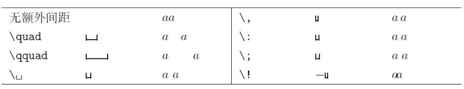
公式中的间距
绝大部分时候,数学公式中各元素的间距是根据符号类型自动生成的,需要手动调整的情况极少。已经认识了两个生成间距的命令
\quad 和
\qquad。在公式中可能用到的间距还包括\,、\:、\;
以及负间距 \!。文本中的 \␣
也能使用在数学公式中。
一个常见的用途是修正积分的被积函数 \(f(x)\) 和微元 \(\mathrm{d}x\) 之间的距离。注意微元里的 \(\mathrm{d}\) 用的是直立体:
1 | \[ |
\[
\int_a^b f(x)\mathrm{d}x
\qquad
\int_a^b f(x)\,\mathrm{d}x
\]
另一个用途是生成多重积分号。如果直接连写两个
\int,之间的间距将会过宽,此时可以使用负间距
\! 修正之。不过 amsmath
提供了更方便的多重积分号,如二重积分
\iint、三重积分\iiint 等。
1 | \newcommand\diff{\,\mathrm{d}} |
\[ \newcommand\diff{\,\mathrm{d}} \begin{gather*} \int\int f(x)g(y) \diff x \diff y \\ \int\!\!\!\int f(x)g(y) \diff x \diff y \\ \iint f(x)g(y) \diff x \diff y \\ \iint\quad \iiint\quad \idotsint \end{gather*} \]
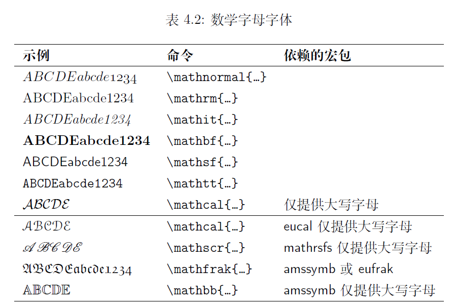
数学符号的字体控制
数学字母字体
\(\LaTeX{}\) 允许一部分数学符号切换字体,主要是拉丁字母、数字、大写希腊字母以及重音符号等。下表给出了切换字体的命令。某些命令需要字体宏包支持。
1 | % \usepackage{amssymb} |
\[ % \usepackage{amssymb} \begin{gather*} \mathcal{R} \quad \mathfrak{R} \quad \mathbb{R} \\ \mathcal{L} = -\frac{1}{4}F_{\mu\nu}F^{\mu\nu} \\ \mathfrak{su}(2) \ and \ \mathfrak{so}(3) \ Lie \ algebra \end{gather*} \]
一般来说,不同的数学字体往往带有不同的语义,如矩阵、向量等常会使用粗体或粗斜体,而数集常会使用
\mathbb
表示。出于内容与格式分离以及方便书写的考虑,可以为它们定义新的命令。
加粗的数学符号
上表中的 \mathbf
命令只能获得直立、加粗的字母。如果想得到粗斜体(国内使用粗斜体符号表示矢量,见
GB/T 3102.11—1993)。可以使用 amsmath 宏包提供的
\boldsymbol 命令:
1 | $\mu, M \qquad \boldsymbol{\mu}, \boldsymbol{M}$ |
\[ \mu, M \qquad \boldsymbol{\mu}, \boldsymbol{M} \]
也可以使用 bm 宏包提供的 \bm 命令:
1 | % \usepackage{bm} |
在 \(\LaTeX{}\)
默认的数学字体中,一些符号本身并没有粗体版本,使用
\boldsymbol 也得不到粗体。此时 \bm
命令会生成“伪粗体”,尽管效果比较粗糙,但在某些时候也不失为一种解决方案。
数学符号的尺寸
数学符号按照符号排版的位置规定尺寸,从大到小包括行间公式尺寸、行内公式尺寸、上下标尺寸、次级上下标尺寸。除了字号有别之外,行间和行内公式尺寸下的巨算符也使用不一样的大小。 为每个数学尺寸指定了一个切换的命令,见 下表。
| 命令 | 尺寸 | 示例 |
|---|---|---|
\displaystyle |
行间公式尺寸 | \(\displaystyle\sum a\) |
\textstyle |
行内公式尺寸 | \(\textstyle\sum a\) |
\scriptstyle |
上下标尺寸 | \(\scriptstyle a\) |
\scriptscriptstyle |
次级上下标尺寸 | \(\scriptscriptstyle a\) |
通过以下示例对比行间公式和行内公式的区别。在分式中,分子分母默认为行内公式尺寸,示例中将分母切换到行间公式尺寸:
1 | \[ |
\[
r = \frac
  {\sum_{i=1}^n (x_i- x)(y_i- y)}
  {\displaystyle \left[
    \sum_{i=1}^n (x_i-x)^2
    \sum_{i=1}^n (y_i-y)^2
  \right]^{1/2} }
\]
定理环境
\(\LaTeX{}\) 原始的定理环境
使用 \(\LaTeX{}\)
排版数学和其他科技文档时,会接触到大量的定理、证明等内容。\(\LaTeX{}\) 提供了一个基本的命令
\newtheorem 提供定理环境的定义:
1 | \newtheorem{theorem environment}{title}[section-level] \\ |
\(\textrm{theorem environment}\) 为定理环境的名称。原始的 \(\LaTeX{}\) 里没有现成的定理环境,不加定义而直接使用很可能会出错。\(\textrm{title}\) 是定理环境的标题(“定理”,“公理”等)。
定理的序号由两个可选参数之一决定,它们不能同时使用:
- \(\textrm{section-level}\) 为章节级别,如 \(\texttt{chapter}\)、\(\texttt{section}\) 等,定理序号成为章节的下一级序号;
- \(\textrm{counter}\) 为用
\newcounter自定义的计数器名称,定理序号由这个计数器管理。
如果两个可选参数都不用的话,则使用默认的与定理环境同名的计数器。
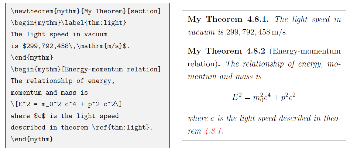
在以下示例代码中,定义了一个 \(\texttt{mythm}\) 环境,其序号设为 \(\texttt{section}\) 的下一级序号。注意 \(\texttt{mythm}\) 环境的可选参数以及
\label 的用法:
1 | \newtheorem{mythm}{My Theorem}[section] |
amsthm 宏包
\(\LaTeX{}\)
默认的定理环境格式为粗体标签、斜体内容、定理名用小括号包裹。如果需要修改格式,则要依赖其它的宏包,如
amsthm、ntheorem 等等。本小节简单介绍一下
amsthm 的用法。
amsthm 提供了 \theoremstyle
命令支持定理格式的切换,在用 \newtheorem
命令定义定理环境之前使用。amsthm
预定义了三种格式用于\theoremstyle:\(\texttt{plain}\) 和 \(\LaTeX{}\) 原始的格式一致;\(\texttt{definition}\)
使用粗体标签、正体内容;\(\texttt{remark}\)
使用斜体标签、正体内容。
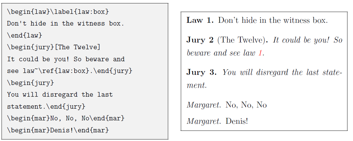
另外 amsthm 还支持用带星号的 \newtheorem*
定义不带序号的定理环境:
1 | \theoremstyle{definition} \newtheorem{law}{Law} |
以上例子定义的 \(\texttt{jury}\) 环境与 \(\texttt{law}\) 环境共用编号,\(\texttt{mar}\) 环境不编号:
1 | \theoremstyle{definition} \newtheorem{law}{Law} |
amsthm 还支持使用 \newtheoremstyle
命令自定义定理格式,更为方便使用的是 ntheorem
宏包。感兴趣的读者可参阅它们的帮助文档。
证明环境和证毕符号
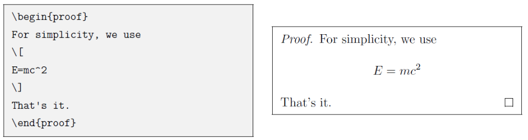
amsthm 还提供了一个 \(\texttt{proof}\)
环境用于排版定理的证明过程。环境末尾自动加上一个 □ 证毕符号:
1 | \begin{proof} |
如果行末是一个不带编号的公式,□ 符号会另起一行,这时可使用
\qedhere 命令将 □ 符号放在公式末尾:
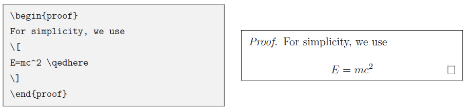
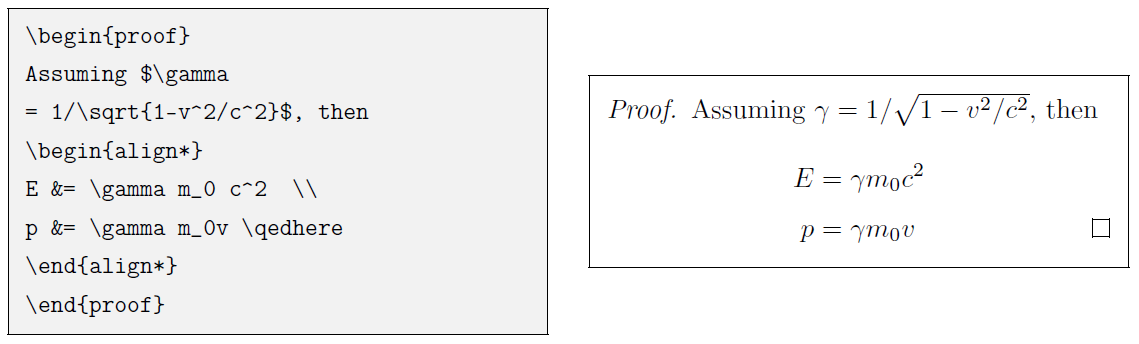
\qedhere 对于 \(\texttt{align*}\) 等环境也有效:
1 | \begin{proof} |
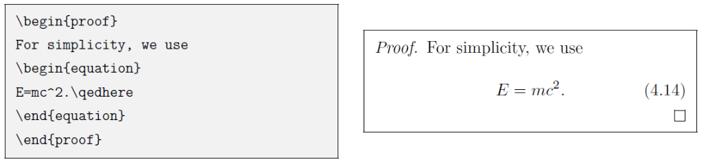
在使用带编号的公式时,最好不要在公式末尾使用
\qedhere 命令。对带编号的公式使用\qedhere
命令会使 □ 符号放在一个难看的位置,紧贴着公式:
在 \(\texttt{align}\) 等环境中使用
\qedhere 命令会使 □ 盖掉公式的编号;使用 \(\texttt{equation}\) 嵌套 \(\texttt{aligned}\)
等环境时,\qedhere 命令会将 □
直接放在公式后。这些位置都不太正常。
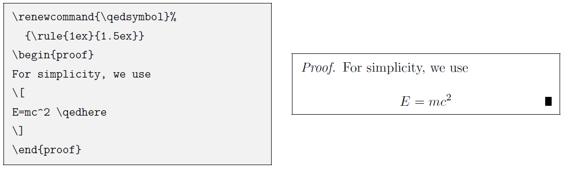
证毕符号 □ 本身被定义在命令 \qedsymbol
中,如果有使用实心符号作为证毕符号的需求,需要自行用
\renewcommand}命令修改。可以利用标尺盒子来生成一个适当大小的“实心矩形”:
1 | \renewcommand{\qedsymbol}% |
符号表
在这里。
参考文献
[1] Partl H, Hyna I, Schlegl E. 一份 (不太) 简短的 LATEX2ε 介绍[J].
2024. https://github.com/CTeX-org/lshort-zh-cn